Maybe you were following the flood risk created 2 years ago by the Hunza Valley landslide in January 2010. There were fears that once the lake overflowed it would trigger a massive outburst flood (you can have a look at my previous post, focused on this phenomenon). More than 25,000 people in Gojal were stuck after the massive landslide formed a natural dam in the Hunza River, creating a lake that consumed upstream villages as it expanded. The landslide also blocked the Karakoram Highway, a vital trade link connecting the region to China.
The spillways need to be blasted (...)The district administration of Hunza Nagar made an announcement last week to blast the spillway on February 18, but put off the task till the 27th of this month.(...)Explosives will be used to blast the boulders currently obstructing the outflow of water though a spillway dug in 2010. Several unsuccessful attempts have been made in the past using controlled blasting to widen the spillway.An official said that traffic on the Gilgit-Hunza portion of the Karakoram Highway would be stopped on that day. Authorities also warned residents settled downstream to avoid venturing to the riverside. Pakistan Red Crescent society (PRCS) has deputed a team of volunteers to assist the administration in case of an emergency.
Let's hope everything is done safely and that the blast serves to get knowledge on how do outburst floods develop.
Update 2012-03-01: Level went down by 7m after works to enlarge the spillway and the reopening by blast last monday. Good news for people living downstream: pamirtimes.net
This has been probably helped by the erosion produced by the peak discharge reached, about 50,000 cusecs (1400 m3/s).
Update 2012-05-15: Another blast of the gravel dam: Pamir Times.
Altai Republic, southern Siberia, close to Mongolia. All the mountains around are older than 60 million years and we are about 300 m above the Chuja River. And yet we are stepping on recent (Pleistocene) gravels! These gravels are similar to those in every river bed except for their elevation above the river and for the fact that they show no apparent stratification: good indications that they were deposited in turbulent waters at that height, only 15 thousand years ago. The problem is: considering the valley width and the slope along the river in this area (~0.6%), such high water should have moved faster than 30 m/s, implying a discharge of about 100 times the present Amazon river. This event is getting to be known as the Altai Flood (+ info in this pdf).
No meteorological event could explain such a huge water discharge, particularly in a small catchment like that of the Chuja River. Instead, Russian geomorphologists came out during the 80's with this explanation: some tens of kilometers upstream (here), a glacier blocked the Chuja River for some thousands of years and formed a large lake behind. When the ice barrier collapsed, the sudden release of the lake's water produced a gigantic outburst flood with no historical precedent. This is today the most accepted interpretation of features such as the gravels laying along the flanks of the Katun valley (e.g., Herget, 2009).
This picture is taken from the top of the gravel deposits, nearly 300 m above today's river level. The gravels (note their size of a few cm) are interpreted to mark the upper reaches of the flooding waters when they encountered the hill obstacle and then ran up converting kinetic energy into potential energy. Location map. Other photos of this fieldtrip here.
But wait, doesn't all this sound a bit pre-geological? Religions often depict the Earth as being shaped by large floods and cataclysms following Creation. Is geology now acknowledging some truth in those myths?
I uploaded to Youtube a simple but interesting numerical model. It computes a constant tectonic uplift with the competing river erosion along a cross section, allowing enough time to reach two successive topographic steady states (one during uplift, another one after uplift):
Steady state topography development, and other parameters of the model.
Uplift occurs between x=-50 and x=+50 km. The dashed line indicates
the topographic profile that would develop in absence of erosion.
Equilibrium topography is reached at ~4 and at ~8 Myr.
This is calculated assuming constant uplift rate at the center (x=-50 to +50 km) and a 1D stream power law erosion model. Uplift rate is 1 mm/yr and stops at t=5 Myr. River erosion is proportional to slope and water discharge. Precipitation rate is constant over the entire profile. Calculations are performed under Linux with the program tAo (Garcia-Castellanos, 2007, EPSL). +info and software download here: https://sites.google.com/site/daniggcc/software/tao
As you can see, topographic growth goes on until a first steady state (with a maximum topography of ~3000 m) is reached before 5 Myr. If you look at the numbers, you'll see an equilibrium between erosion rates and uplift rates at that time. At 5 Myr uplift stops and then erosion leads to the new equilibrium: a flat topography (at 8 Myr).
Now, the question is: does steady-state topography exist in nature? And if it does, can we recognize it? In real Earth, neither climate nor tectonics are constant through time. The questions are probably too big for this small blog, but you can find some hints in this article by Willett and Brandon (2001).
Nevertheless, the notion of steady-state topography is useful to understand some basic principles of orogenesis, as Whipple (2009) showed in a very simple and elegant way. Consider these two end-member types of orogen:
Evolution of for parameters (orogen width, erosion, topography, and rock uplift) for two simple models of orogenic growth. Left: fixed width orogen; Right: Self-similar growth. At t=0, the erosion coefficient is set to a double value (red) and to half of the reference value (green). Erosion is assumed proportional to elevation. The parameters are shown normalized. Redrawn from Whipple (2009).
Assume both orogens grow in response to the convergence of two tectonic plates, producing a constant tectonic flow Fa, and that they are eroded at a rate proportional to elevation. The red lines in the figures above correspond to a change to double erosion efficiency. With such a simple representation, it becomes clear that if erosion mechanisms become more efficient, both orogen types initially undergo an increase in erosion rate, but this will gradually decrease back to the initial erosion value (the one compensating the imposed tectonic flow, as in the animation above). The way the orogen returns to the original low erosion rate is by decreasing its elevation R.
One interesting thing is that, whereas for a fixed width, rock uplift rates return to normal after some time, the self-similar growth predicts a permanent increase in uplift rates.
And the other interesting conclusion is that the time response is controlled mainly by the erosion efficiency itself (within the approaches of the model, of course).
Simple models are generally more inspiring than the most complex ones.
References:
Whipple, K. (2009). The influence of climate on the tectonic evolution of mountain belts Nature Geoscience, 2 (2), 97-104 DOI: 10.1038/ngeo413
Willett, S., and Brandon, M. (2001). On steady states in mountain belts Geology, 30, 175-178
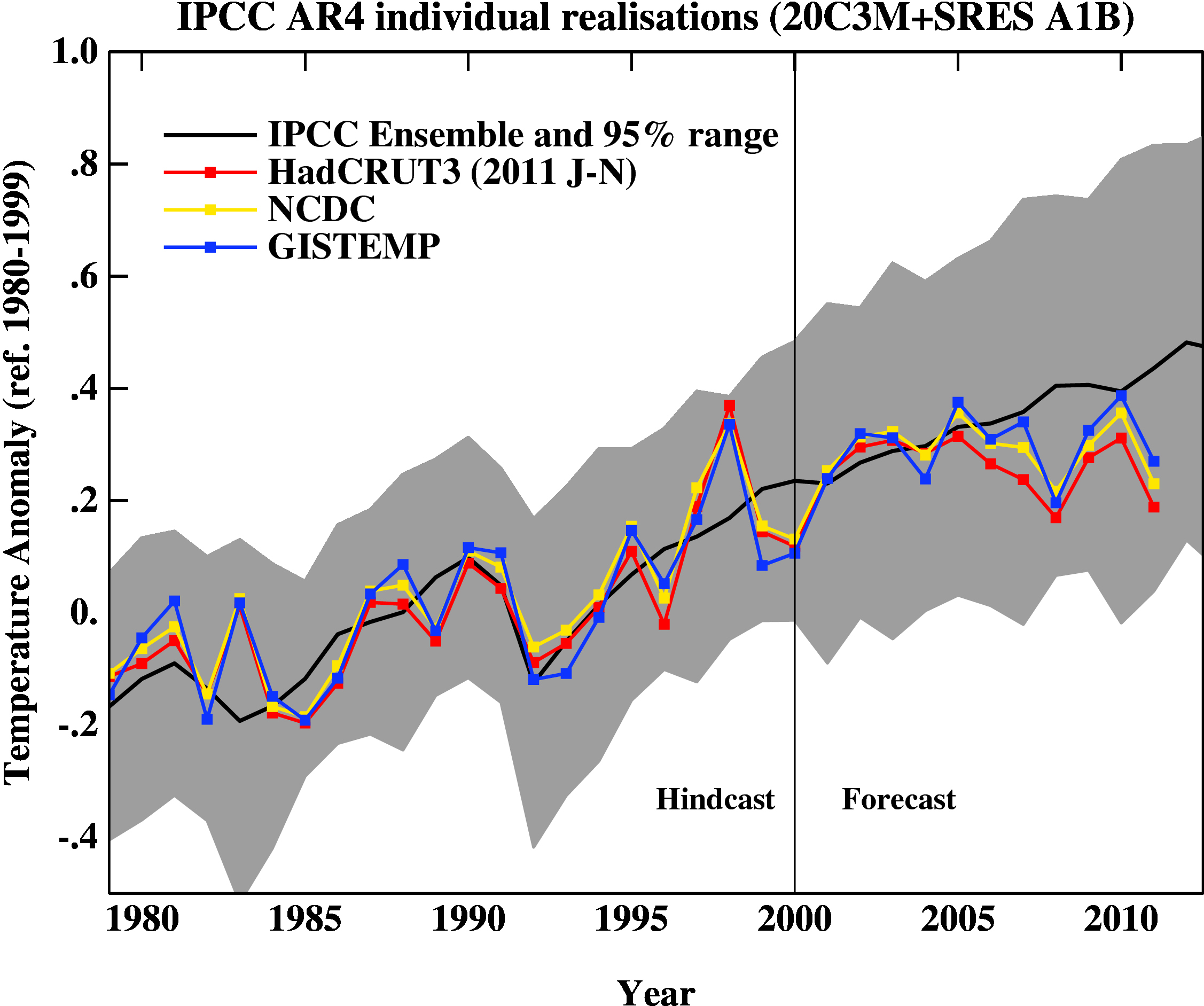
Curious about the global temperature trend after updating with last-years temperature record?
Mean-temperature rise since 1980
Mean anomalies from the IPCC AR4 models plotted on surface temperature records (HadCRUT3v, NCDC and GISTEMP). Everything is baselined to 1980-1999 and the envelope in grey encloses 95% of the model runs.
The La Niña event in 2011 cooled the year relative to 2010. Differences between the observational records are mostly related to interpolations in the Arctic. Given current indications of only mild La Niña conditions, 2012 will likely be a warmer year than 2011, so again another top 10 year, but not a record breaker – that will have to wait until the next El Niño.
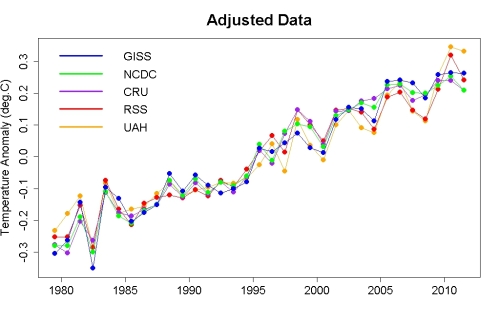
Corrected for short-term processes
Foster and Rahmstorf (2011) showed nicely that if you account for some of the obvious factors affecting the global mean temperature (such as El Niños/La Niñas, volcanoes etc.) there is a strong and continuing increasing trend. An update to that analysis using the latest data is available here.
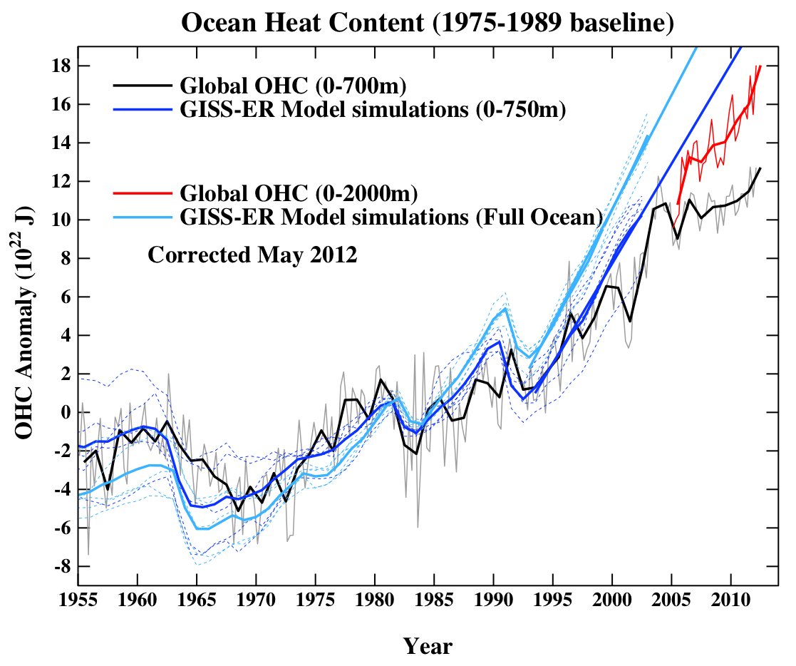
Ocean Heat Content
Ocean heat content (OHC) in the models compared to the latest data from NODC. All curves are baselined to the period 1975-1989.
Summer sea ice changes
Sea ice changes this year were dramatic, with the Arctic September minimum reaching record values (depending on the data product). Updating the Stroeve et al, 2007 analysis (courtesy of Marika Holland) using the NSIDC data we can see that the Arctic continues to melt faster than any of the AR4/CMIP3 models predicted.